DP

DP Model

Tutorial

DP Model Overview

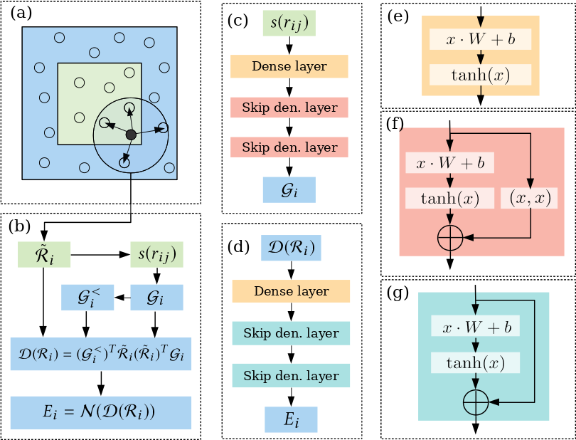
For the DP model, see the following references:

• [SC’20] Weile Jia, Han Wang, Mohan Chen, Denghui Lu, Lin Lin, Roberto Car, E Weinan, Linfeng Zhang*, "Pushing the Limit of Molecular Dynamics with Ab Initio Accuracy to 100 Million Atoms with Machine Learning," SC20: International Conference for High Performance Computing, Networking, Storage and Analysis, 2020, pp. 1-14, doi: 10.1109/SC41405.2020.00009.(CCF-A)(Gordon Bell Prize)

• Han Wang, Linfeng Zhang, Jiequn Han, and Weinan E. "DeePMD-kit: A deep learning package for many-body potential energy representation and molecular dynamics." Computer Physics Communications 228 (2018): 178-184. doi:10.1016/j.cpc.2018.03.016

• Zhang L, Han J, Wang H, et al. End-to-end symmetry preserving inter-atomic potential energy model for finite and extended systems[J]. Advances in neural information processing systems, 2018, 31.

• Lu D, Jiang W, Chen Y, et al. DP compress: A model compression scheme for generating efficient deep potential models[J]. Journal of chemical theory and computation, 2022, 18(9): 5559-5567.

type embedding

A DP model contains $N^2$ Embedding Nets, where $N$ is the number of element types. When a system contains many element types, this design limits both training and inference speed and restricts the potential of DP as a general-purpose large model. Because the $N^2$ Embedding Nets implicitly encode element types, we modify $S_{ij}$ by concatenating it with the physical properties of the corresponding element type. This enables a single Embedding Net to achieve results comparable to those of $N^2$ networks.

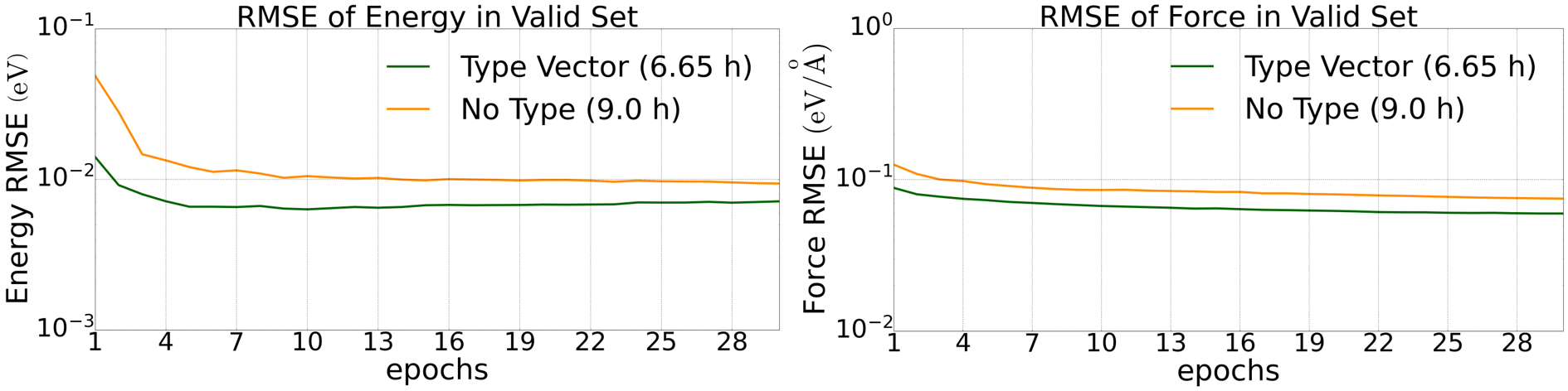
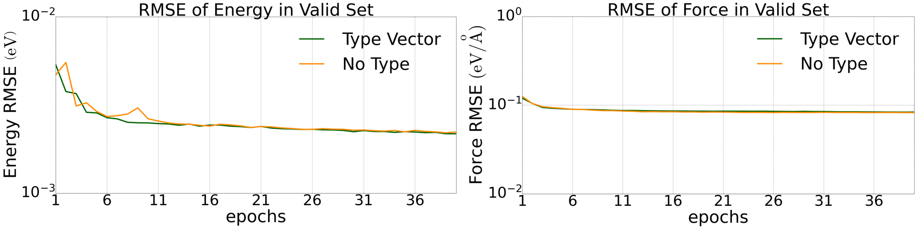
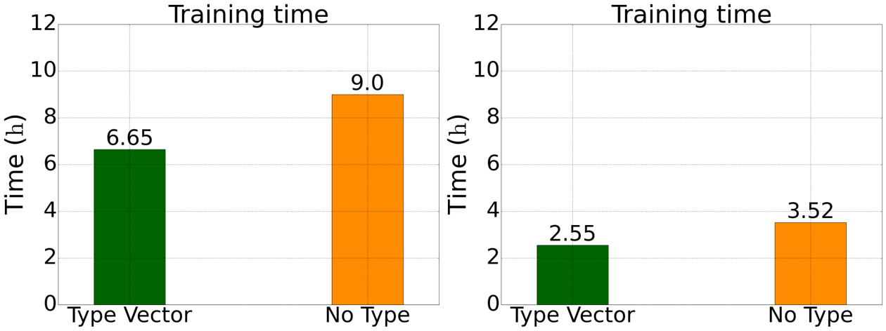
For $S_{ij}$, $i$ is the central atom. The physical properties of the element type corresponding to $j$ are concatenated with $S_{ij}$ to form a vector of length $1 +$ the number of physical properties, which is then passed to the Embedding Net. Tests on our five-component alloy (Ru, Rh, Ir, Pd, and Ni) dataset and quaternary LiGePS dataset (1200 K) show that a DP model using this type-embedding method matches or exceeds the prediction accuracy of a standard DP model while reducing training time by 27%. See the performance benchmarks for details.

Usage

To enable type embedding with the default physical properties, add the $type\_embedding$ parameter to the JSON training configuration. See example/LiGePS/ligeps.json in the project examples.

{
  "type_embedding": true
}

You can also specify the required physical properties in the model parameters of the JSON file.

Performance Benchmark: Accuracy

Comparison of validation-set prediction accuracy between the type-embedding method and a standard DP model on the mixed five-component alloy dataset (9,486 configurations):

Comparison of validation-set prediction accuracy between the type-embedding method and a standard DP model on the quaternary LiGePS dataset (10,000 configurations at 1200 K):

Performance Benchmark: Training Time

The force field is invoked in LAMMPS in the same way as the standard DP model described above.

Polynomial Model Compression

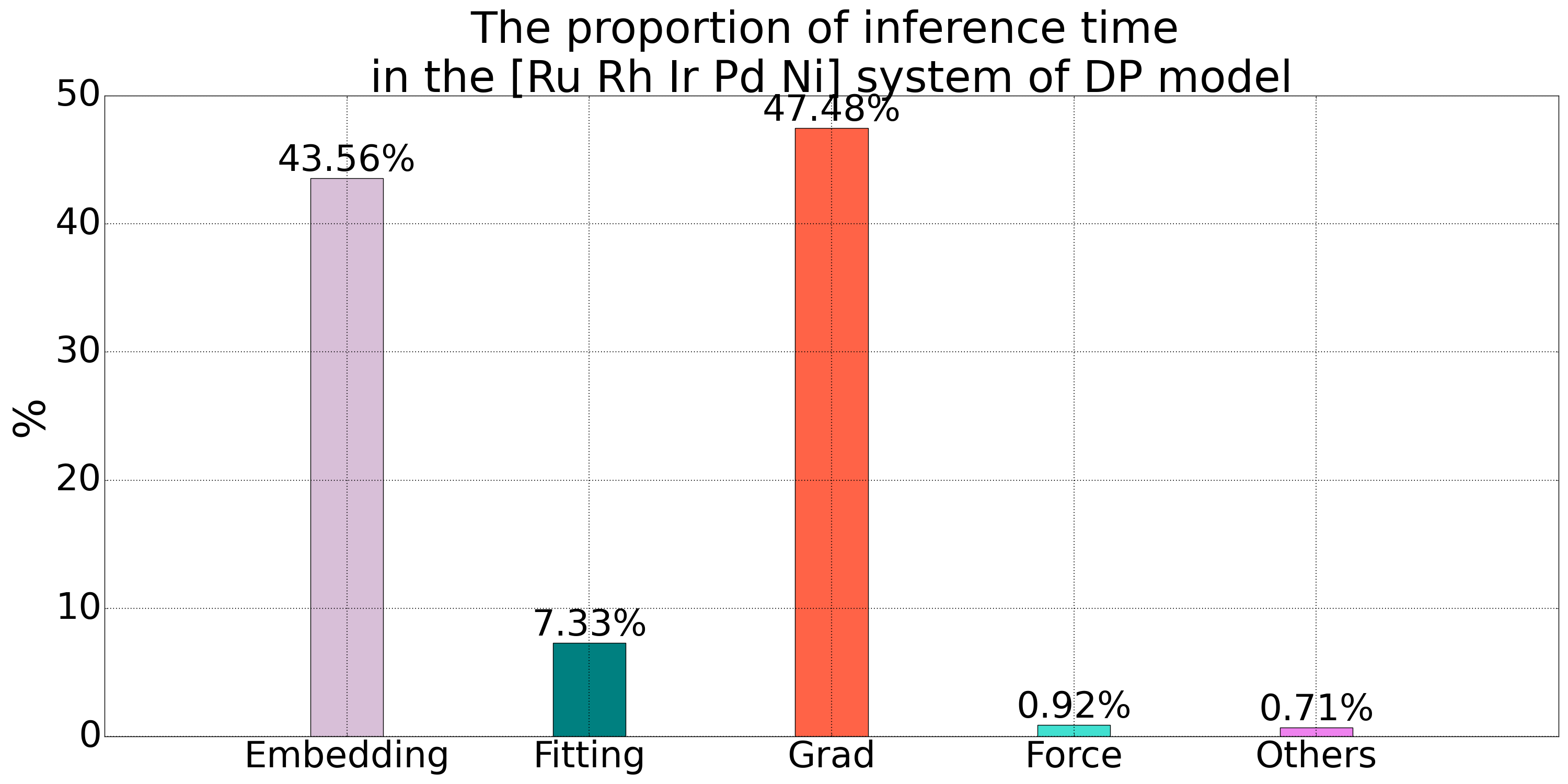
A DP model contains $N^2$ Embedding Nets, where $N$ is the number of atom types. As the number of types increases, the number of Embedding Nets grows rapidly, enlarging the computational graph used for backpropagation and becoming an inference bottleneck. The timing breakdown below for DP inference on a five-component alloy shows that Embedding Net evaluation and gradient computation account for more than 90% of the total time, leaving substantial room for optimization. An Embedding Net takes a scalar $S_{ij}$ as input and outputs $m$ values, where $m$ is the number of neurons in its final layer. It can therefore be replaced by $m$ scalar functions.

MatPL implements the fifth-order polynomial compression method described in Lu D, Jiang W, Chen Y, et al., DP compress: A model compression scheme for generating efficient deep potential models. It also provides a third-order polynomial method based on Hermite interpolation.

Usage

To compress a trained DP model, use the following command:

MatPL compress dp_model.ckpt -d 0.01 -o 3 -s cmp_dp_model

• compress is the compression command.
• dp_model.ckpt is the required model file to compress.
• -d sets the grid spacing for $S_{ij}$; the default is 0.01.
• -o sets the compression order: 3 for third order or 5 for fifth order. The default is 3.
• -s sets the compressed model name. The default is cmp_dp_model.

After compression, the model is used for molecular-dynamics simulations in LAMMPS in the same way as a standard DP model.

Model compression accuracy

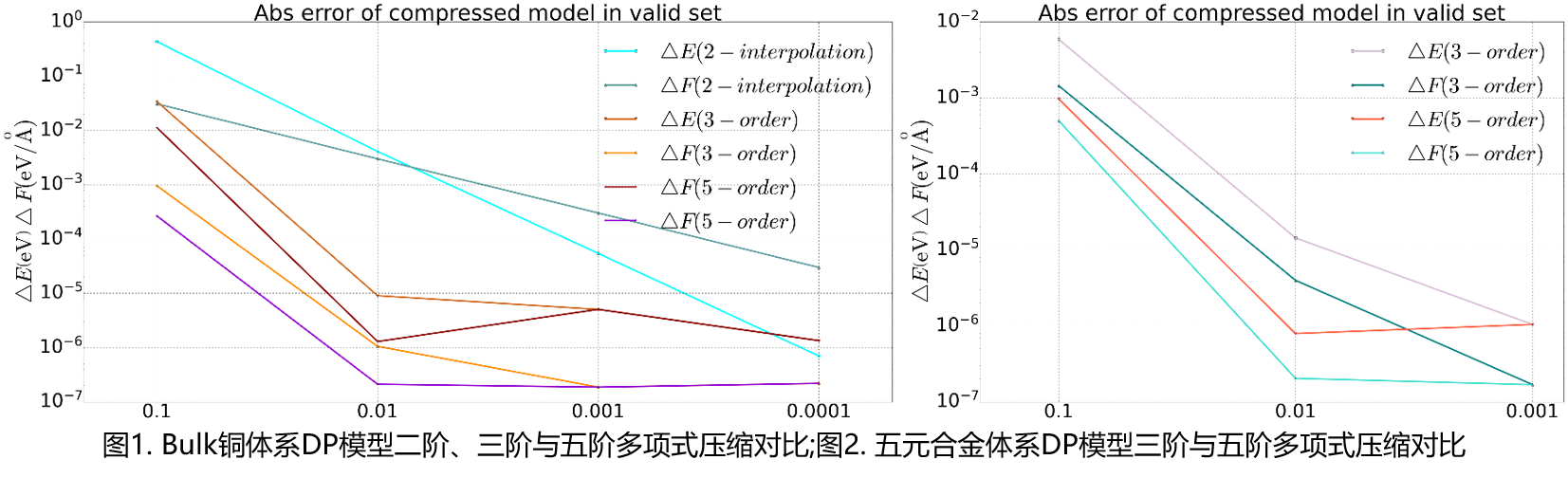
We compressed DP models for bulk copper and a five-component alloy and evaluated them on their respective test sets. The results are shown below. For copper, second-order interpolation is included for comparison; unlike the third- and fifth-order methods, it does not provide sufficient accuracy.

Polynomial Model Compression Procedure

Grid Construction

We scan the entire training set to obtain the maximum value of $s_{ij}$. Because $s_{ij}$ is a function of the three-dimensional distance $r_{ij}$ between atoms $i$ and $j$, it reaches its minimum when $r_{ij} = r_{\text{cut}}$. The range of $s_{ij}$ is divided into $L$ equal intervals of width $dx$, yielding $L+1$ interpolation points denoted by $x_1, x_2, \cdots, x_{L+1}$. In practice, an incomplete training set may not cover every $s_{ij}$ encountered during inference. The grid is therefore extended from the original upper limit to $10 \times s_{ij}$ using a spacing of $10 \times dx$.

Third-Order Polynomial

For each interval $[x_l, x_{l+1})$, the Embedding Net is replaced by the following third-order polynomial:

$$g^l_m(x) = a^l_m x^3 + b^l_m x^2 + c^l_m x + d^l_m$$

Here, $m$ is the number of neurons in the final layer of the Embedding Net—that is, the number of output values—and the polynomial variable $x$ is $s_{ij} - x_l$. The following two conditions must hold at every grid point:

1. The polynomial value equals the Embedding Net output:

   $$y_l = \mathcal{G}_m(x_l)$$

2. The first derivative of the polynomial equals the first derivative of the Embedding Net with respect to $s_{ij}$:

   $$y'_l = \mathcal{G}'_m(x_l)$$

The resulting coefficients are

$$a^l_m = \frac{1}{\Delta t^3} \left[ (y'_{l+1} + y'_l) \Delta t - 2h \right]$$ $$b^l_m = \frac{1}{\Delta t^2} \left[ -(y'_{l+1} + 2y'_l) \Delta t + 3h \right]$$ $$c^l_m = y'_l$$ $$d^l_m = y_l$$

where $h = y_{l+1} - y_l$ and $\Delta t = x_{l+1} - x_l$.

Fifth-Order Polynomial

We also implement the fifth-order polynomial compression method from DP Compress.

For the fifth-order polynomial, $s_{ij}$ is partitioned in the same way as for the third-order method, and the Embedding Net is replaced by the following polynomial:

$$g^l_m(x) = a^l_m x^5 + b^l_m x^4 + c^l_m x^3 + d^l_m x^2 + e^l_m x + f^l_m$$

Note that the polynomial variable $x$ is $s_{ij} - x_l$. The following three conditions must hold at every grid point:

1. The polynomial value equals the Embedding Net output:

   $$y_l = \mathcal{G}_m(x_l)$$

2. The first derivative of the polynomial equals the first derivative of the Embedding Net with respect to $s_{ij}$:

   $$y'_l = \mathcal{G}'_m(x_l)$$

3. The second derivative of the polynomial equals the second derivative of the Embedding Net with respect to $s_{ij}$:

   $$y''_l = \mathcal{G}''_m(x_l)$$

The six coefficients are therefore:

$$a^l_m = \frac{1}{2\Delta t^5} \left[ 12h - 6(y'_{l+1} + y'_l) \Delta t + (y''_{l+1} - y''_l) \Delta t^2 \right]$$ $$b^l_m = \frac{1}{2\Delta t^4} \left[ -30h + (14y'_{l+1} + 16y'_l) \Delta t + (-2y''_{l+1} + 3y''_l) \Delta t^2 \right]$$ $$c^l_m = \frac{1}{2\Delta t^3} \left[ 20h - (8y'_{l+1} + 12y'_l) \Delta t + (y''_{l+1} - 3y''_l) \Delta t^2 \right]$$ $$d^l_m = \frac{1}{2} y''_l$$ $$e^l_m = y'_l$$ $$f^l_m = y_l$$

where $h = y_{l+1} - y_l$ and $\Delta t = x_{l+1} - x_l$.

Verification of the Model Compression Formula

The model-compression scheme divides the range of $s_{ij}$ into $L$ equal intervals, giving $L+1$ interpolation points denoted by $x_1, x_2, \cdots, x_{L+1}$. For each interval $[x_l, x_{l+1})$, the embedding network is replaced by the following fifth-order polynomial:

$$g^l_m(x) = a^l_m x^5 + b^l_m x^4 + c^l_m x^3 + d^l_m x^2 + e^l_m x + f^l_m$$

Note that the polynomial variable $x$ is $s_{ij} - x_l$. The following three boundary conditions must hold at every grid point:

1. The function values are equal:

   $$y_l = \mathcal{G}_m(x_l)$$

2. The first derivatives are equal:

   $$y'_l = \mathcal{G}'_m(x_l)$$

3. The second derivatives are equal:

   $$y''_l = \mathcal{G}''_m(x_l)$$

The six coefficients are therefore:

$$a^l_m = \frac{1}{2\Delta t^5} \left[ 12h - 6(y'_{l+1} + y'_l) \Delta t + (y''_{l+1} - y''_l) \Delta t^2 \right]$$ $$b^l_m = \frac{1}{2\Delta t^4} \left[ -30h + (14y'_{l+1} + 16y'_l) \Delta t + (-2y''_{l+1} + 3y''_l) \Delta t^2 \right]$$ $$c^l_m = \frac{1}{2\Delta t^3} \left[ 20h - (8y'_{l+1} + 12y'_l) \Delta t + (y''_{l+1} - 3y''_l) \Delta t^2 \right]$$ $$d^l_m = \frac{1}{2} y''_l$$ $$e^l_m = y'_l$$ $$f^l_m = y_l$$

where $h = y_{l+1} - y_l$ and $\Delta t = x_{l+1} - x_l$.